NOTES: for IGLU environment, we can test
- Winner model
- Decision Transformer
- Modular RL agent
Background
we consider a multitask problem in shared environment
This environment is specified by a tuple
$(S, A, P, \gamma)$, with $S$ a set of states, $A$ a set of low-level actions (actions are common and shared in multitasks)
$P: S\times A\times S \rightarrow \mathbb R$ is a transition probability distribution,
$\gamma$ is a discount factor.
for each task $\tau \in \mathcal T$ is then specified by a pair $(R_{\tau}, \rho _\tau)$ with $R$ a special reward function and $\rho$ an initial distribution over states.
And we assume that tasks are annotated with sketches $K_\tau$, each task sketches consists of a sequence $(b_{\tau 1},b_{\tau 2},b_{\tau 3},…)$ of high-level symbolic labels drawn from a fixed vocabulary $\mathcal B$
Model
constructing for each sketch $b$ a corresponding sub-policy $\pi_b$
this sub-policy $\pi_b$ is shared over multitasks.
- so the author believed that by sharing each policy across all tasks, this approach naturally learns the shared abstraction for the corresponding subtasks.
at each time step $t$, a subpolicy may select ether a low-level action $a \in A$ or a special STOP action.
- potential issue
- agent’s actions are composed in a very complex way, e.g., in IGLU, the agent moves its viewsight, walks and put building blocks in the same time.
- so it is quite hard to split the IGLU task into concrete, non-overlapping sub-tasks.
- Solution: can we just allow policy overlapping ???
this framework is agnostic to the implementation of subpolicies:
- it means that for different sub-policies, we can use different architecture
- e.g., use classical planning for navigation sub-policy
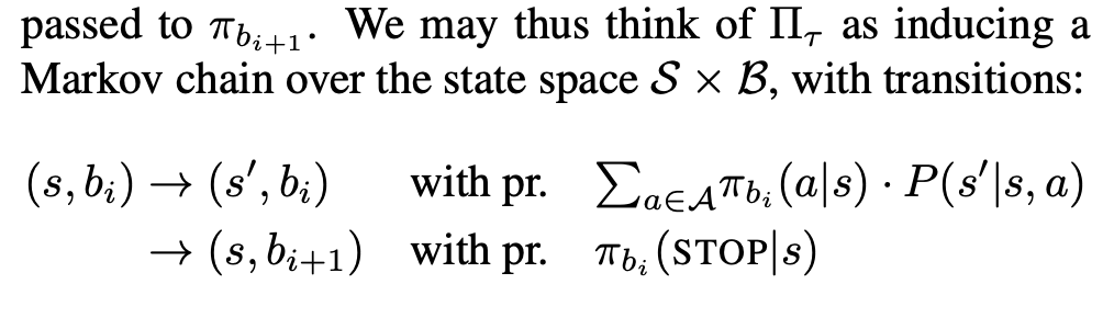
control is passed from $\pi_{b_{i}}$ to $\pi_{b_{i+1}}$ when STOP signal is emitted.
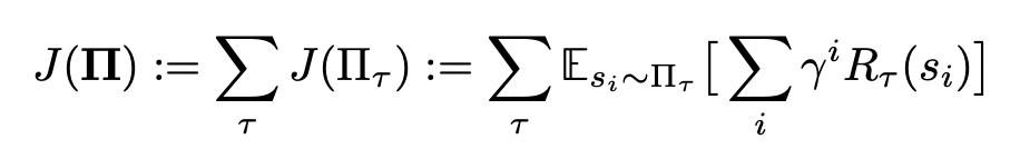
The learning problem is to optimize over all $\theta_b$ to maximise expected discounted reward
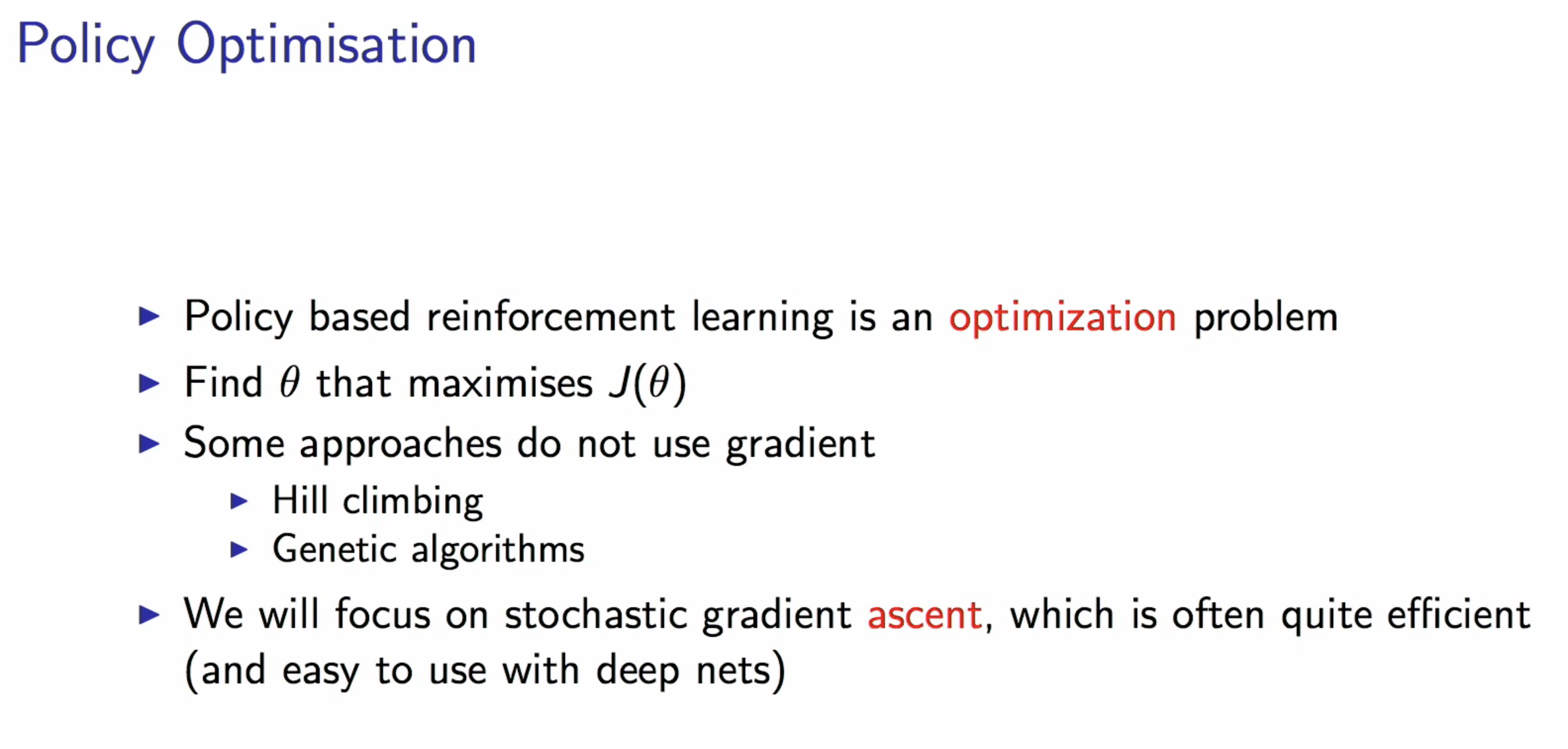
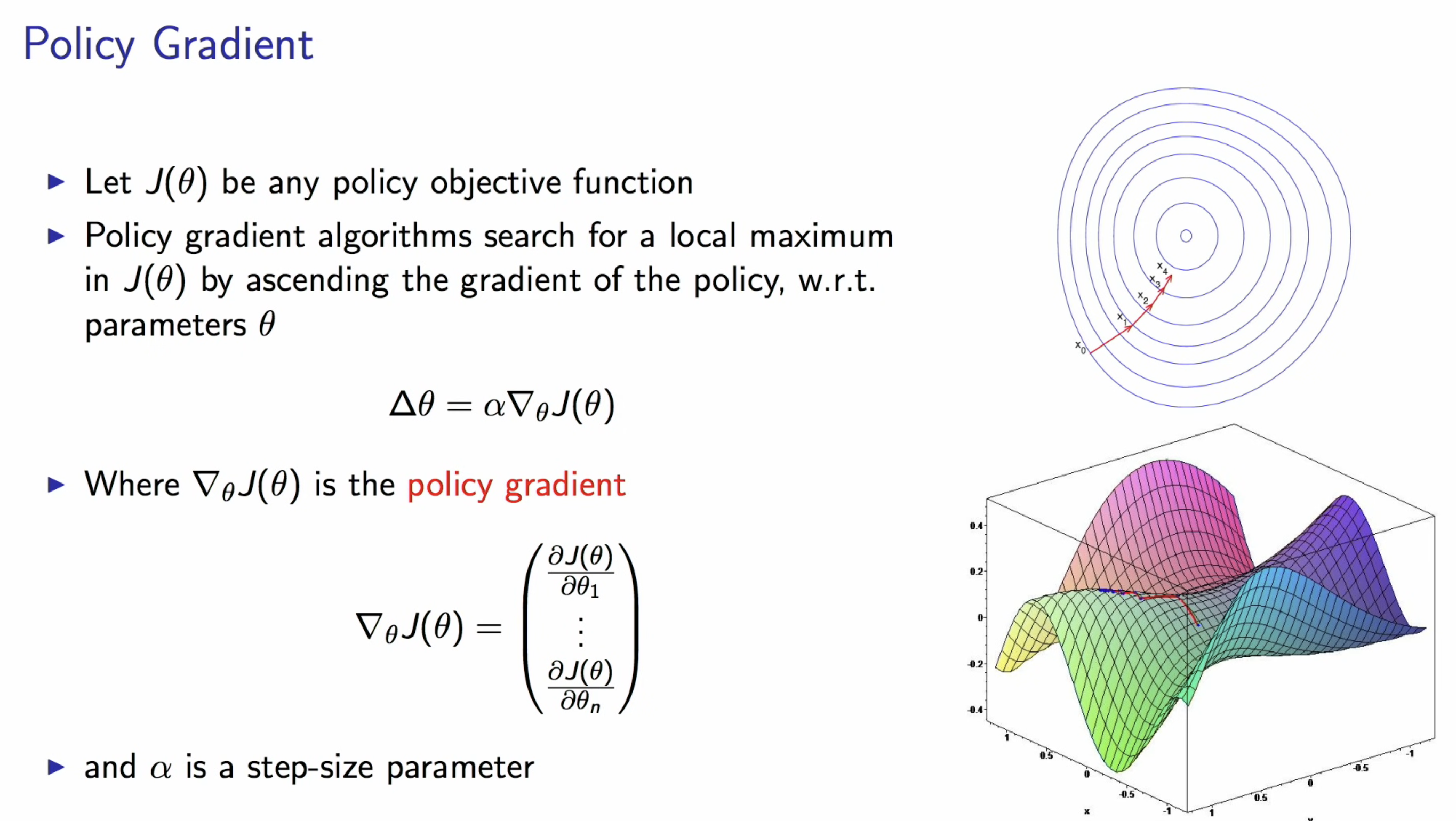
Policy Optimisation
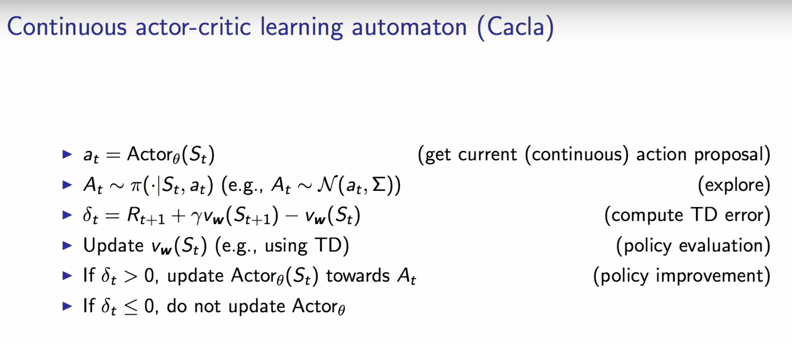
Actor - critic method
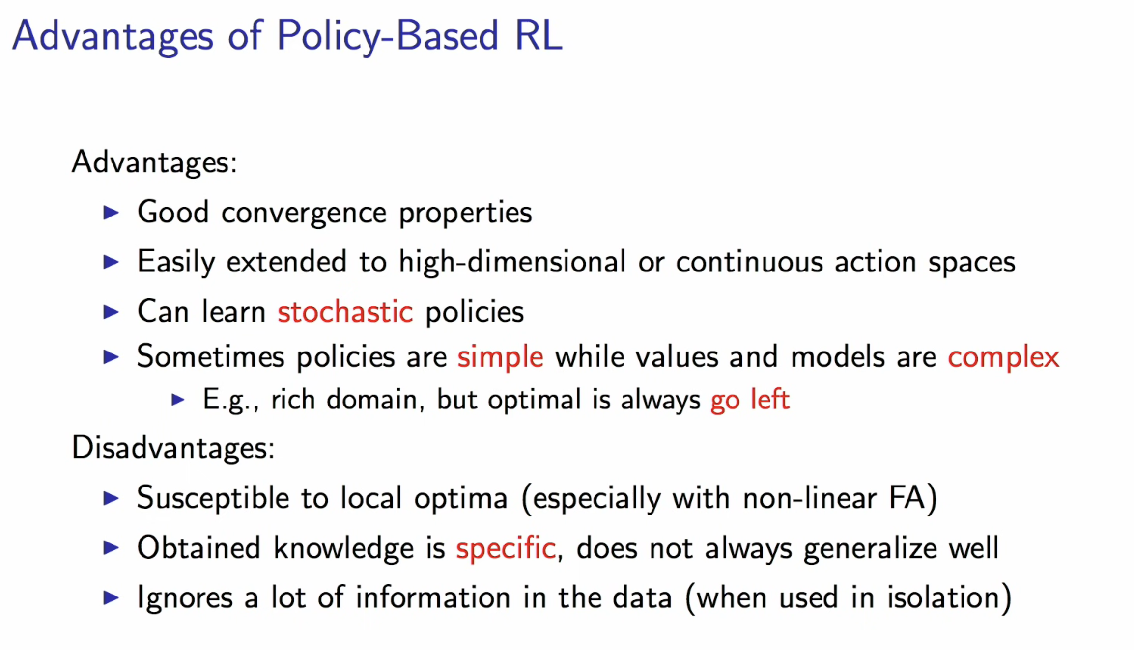
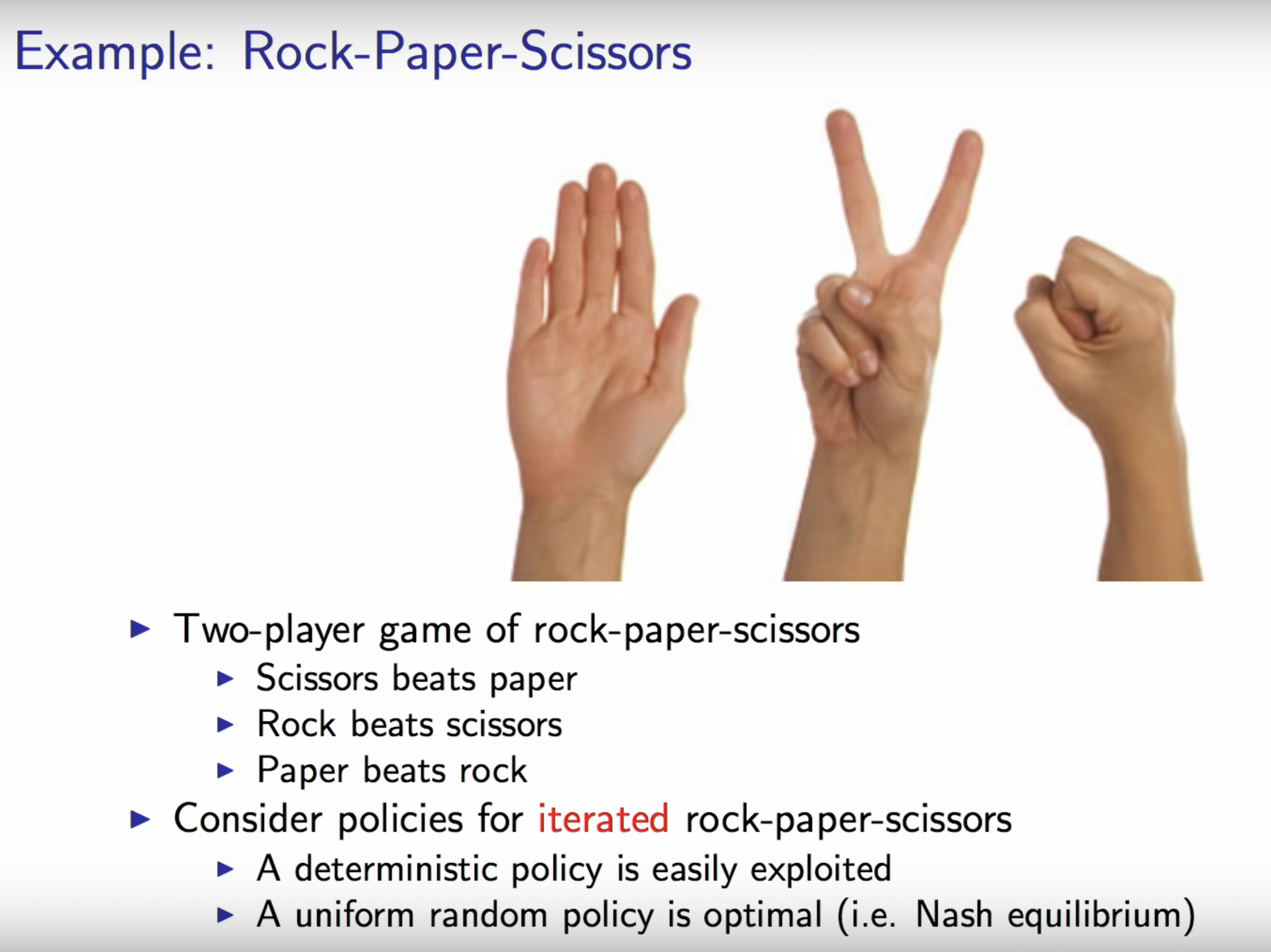
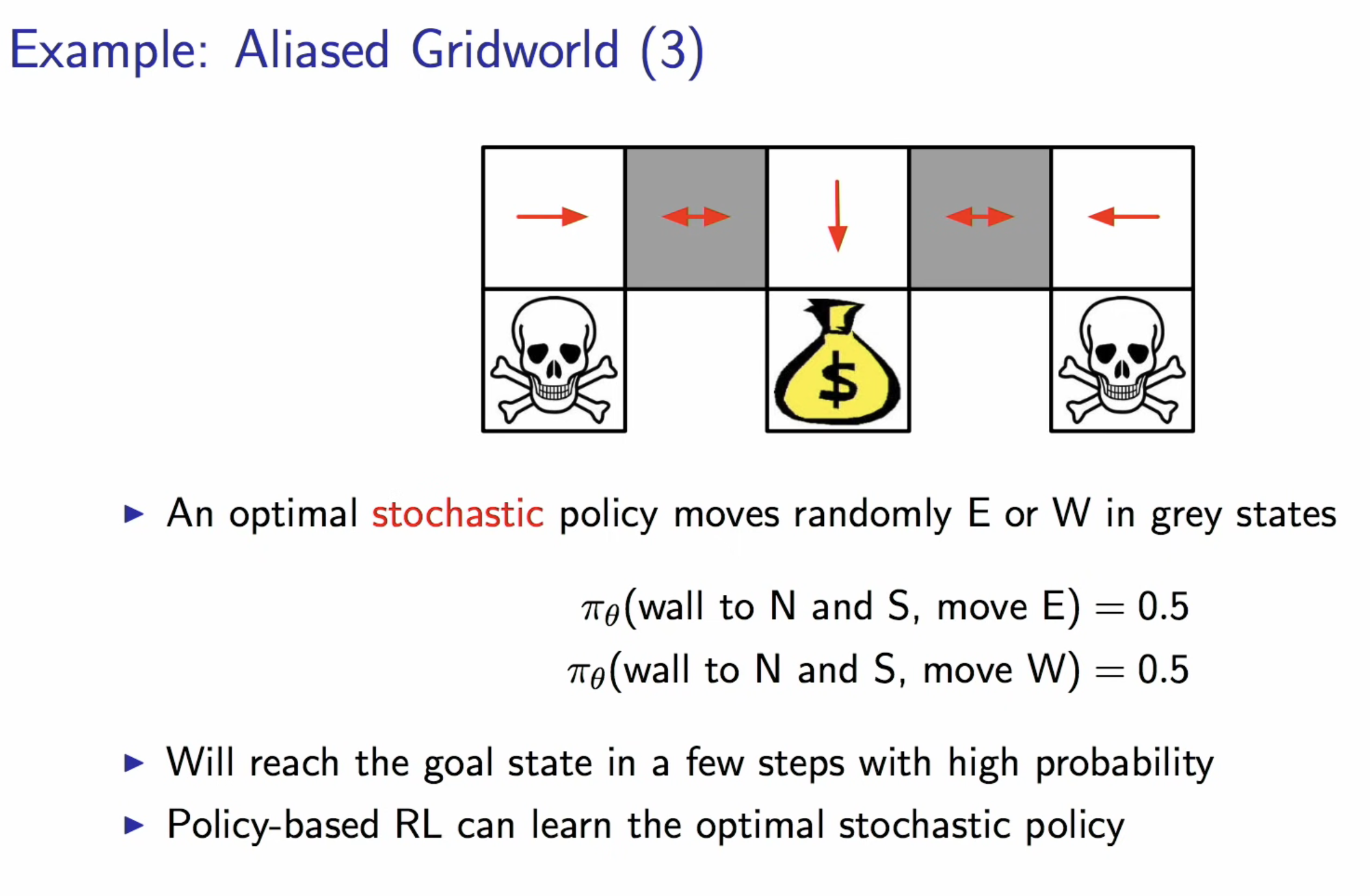
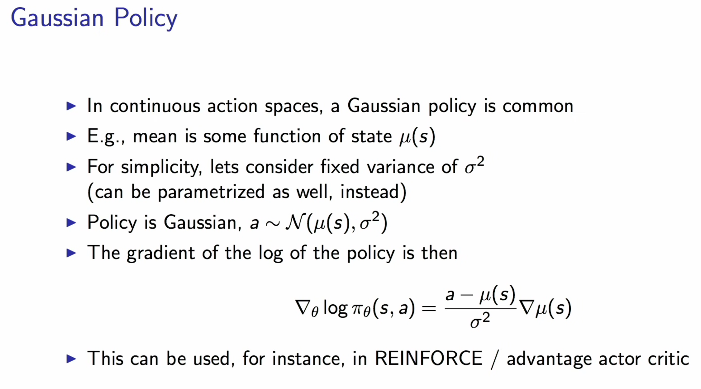
Policy-based RL supports stochastic policy which is good in some cases
So what objectives we want to optimised
- again, maximise the accumulative reward
- or maximise the value of the states
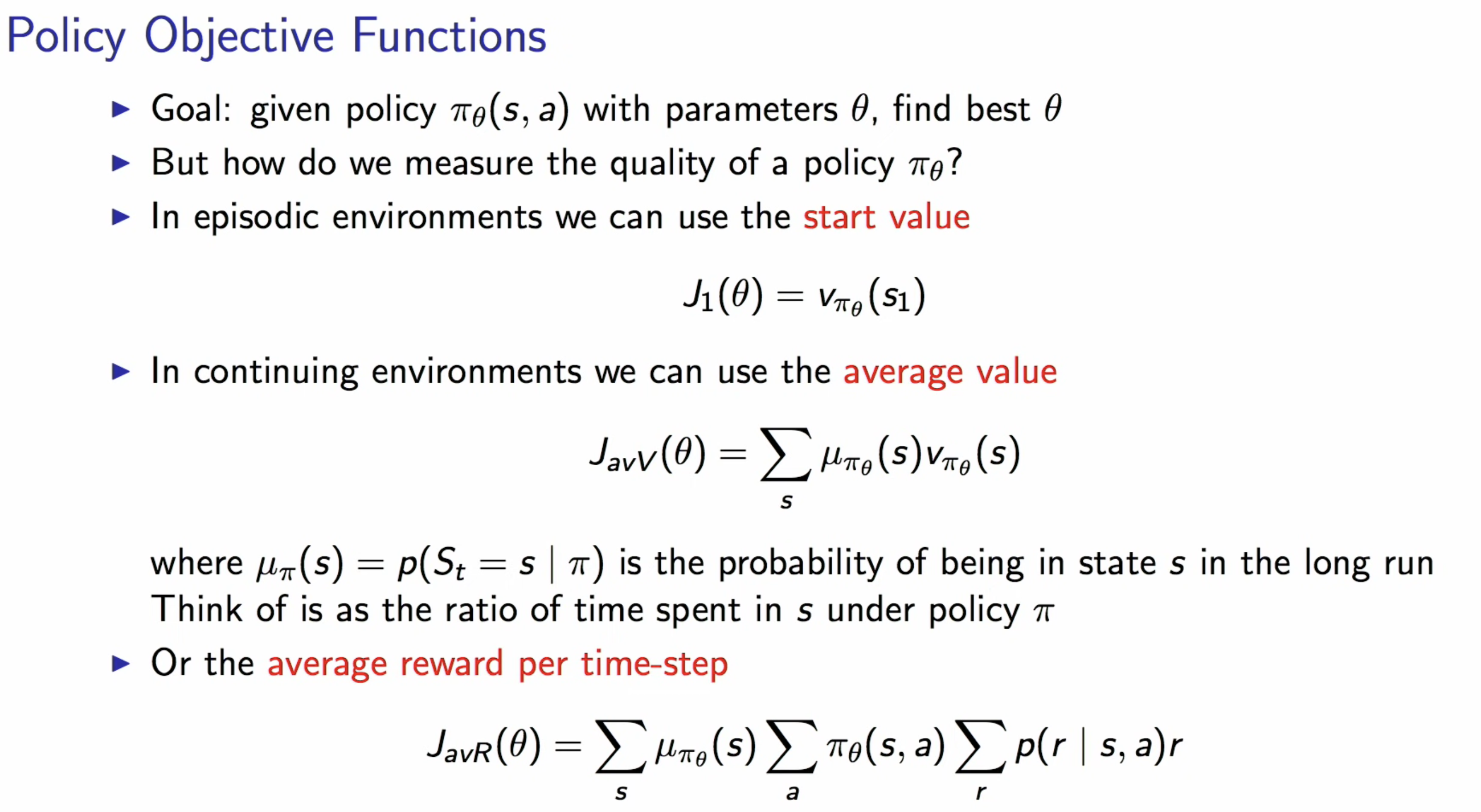
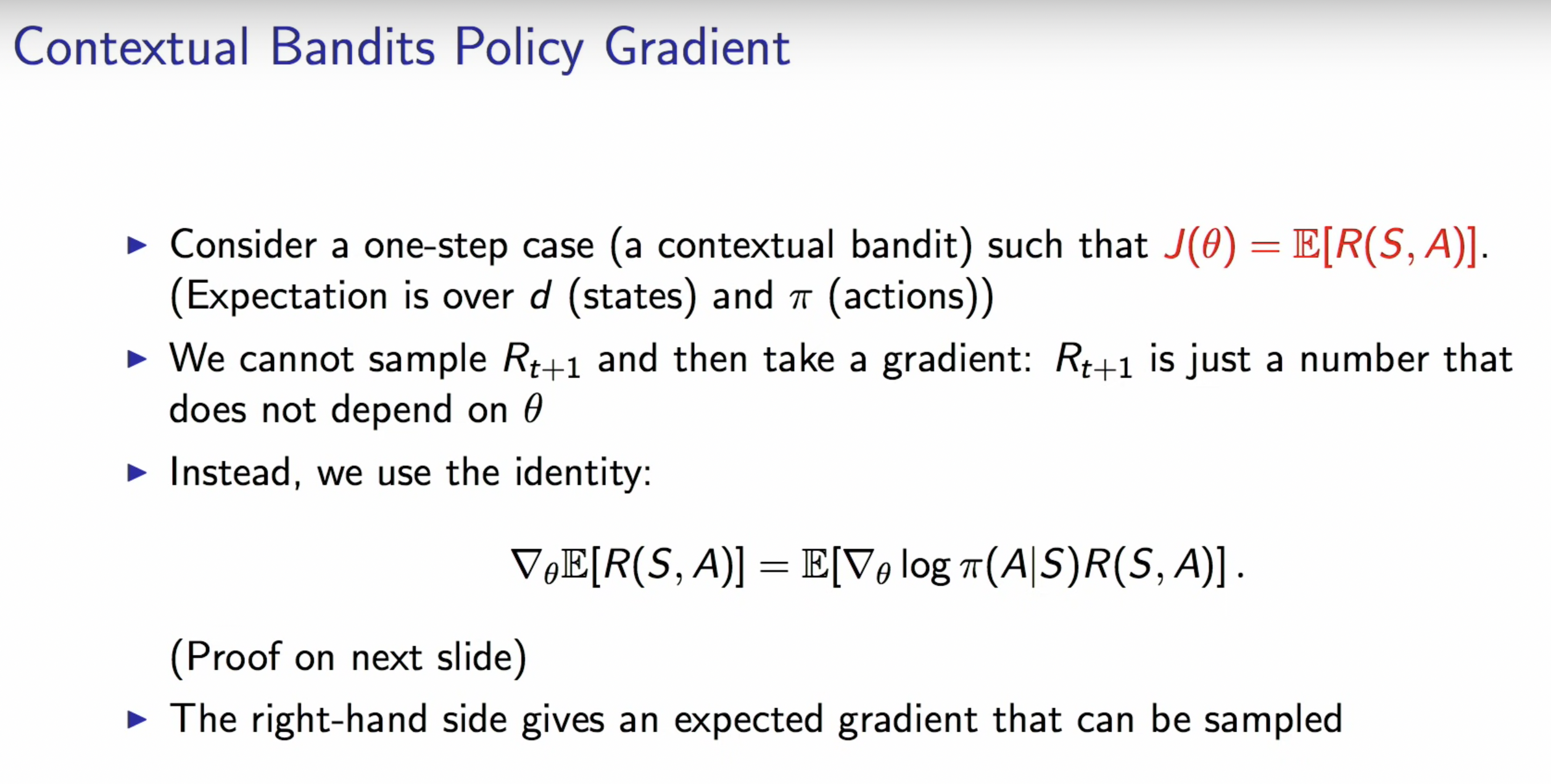
average reward per time-step -> you may want to accumulate it / or just maximise the final reward
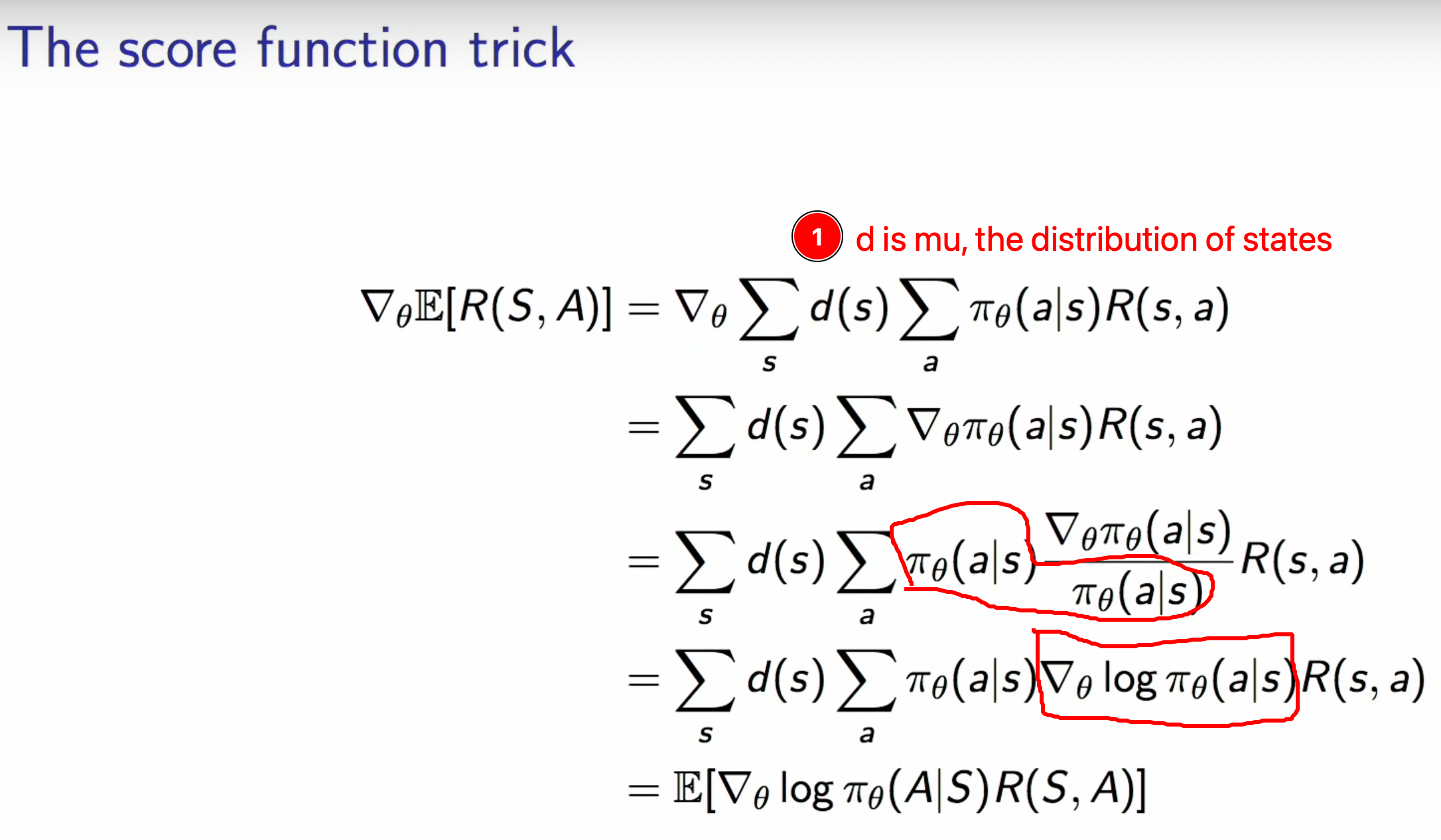
actually, the $\mu$ distribution is the time ratio that we would stay in the states based on current policy
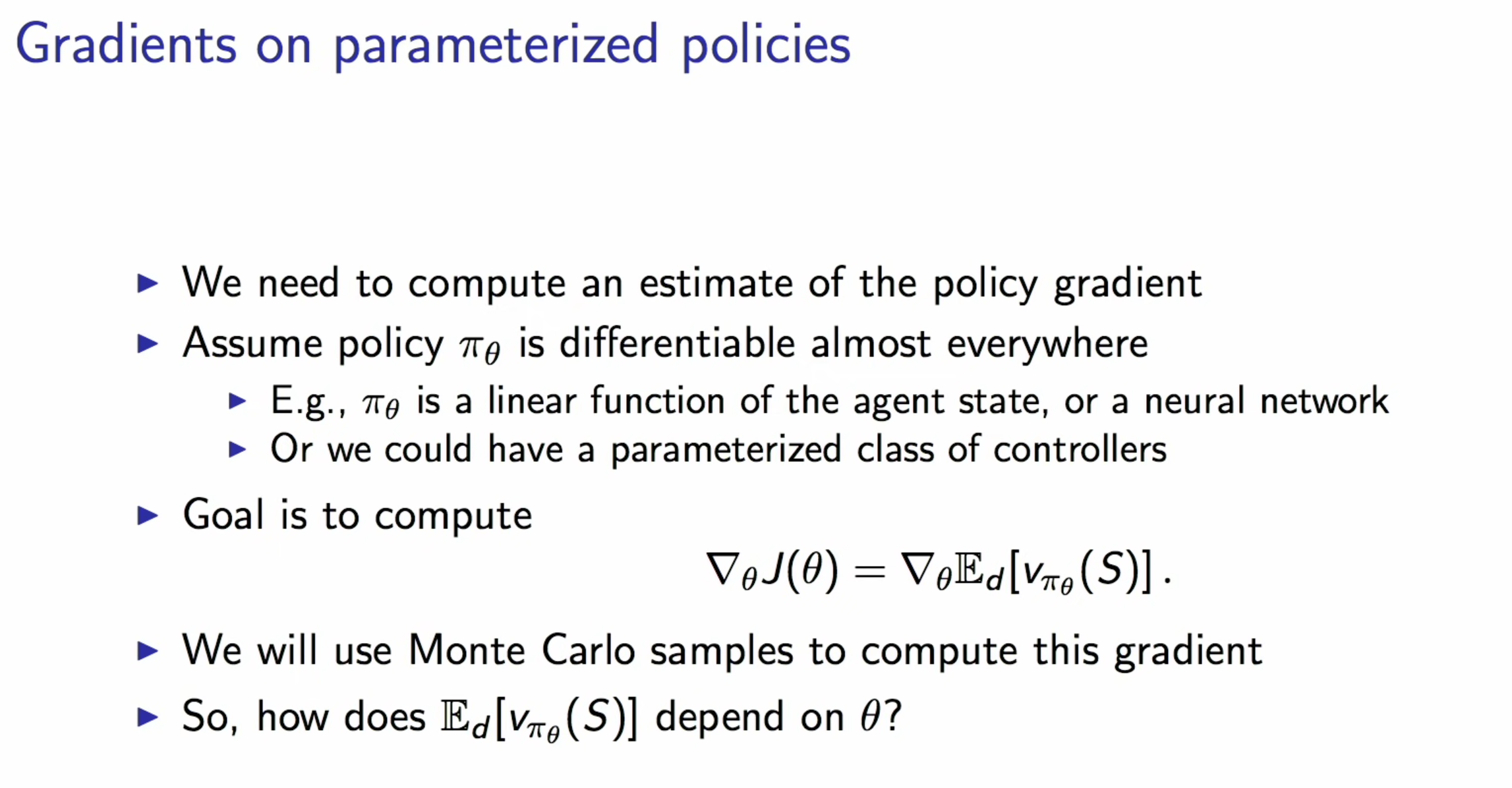
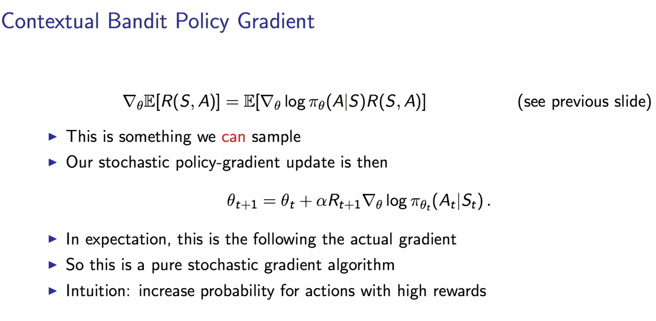
All the slides above is focusing on immediate reward, but we want to extend it to accumulative reward (a.k.a. value of states)
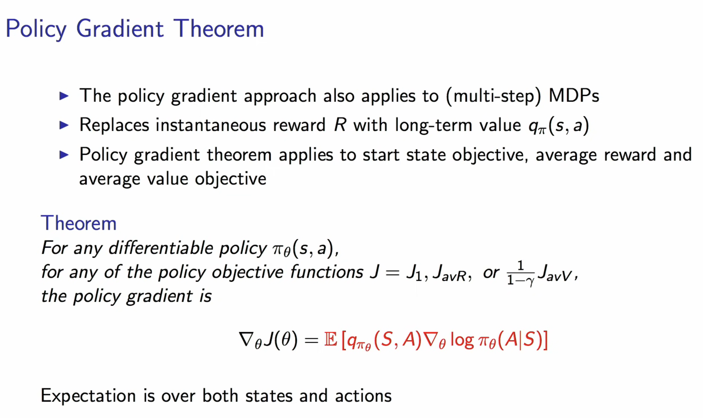
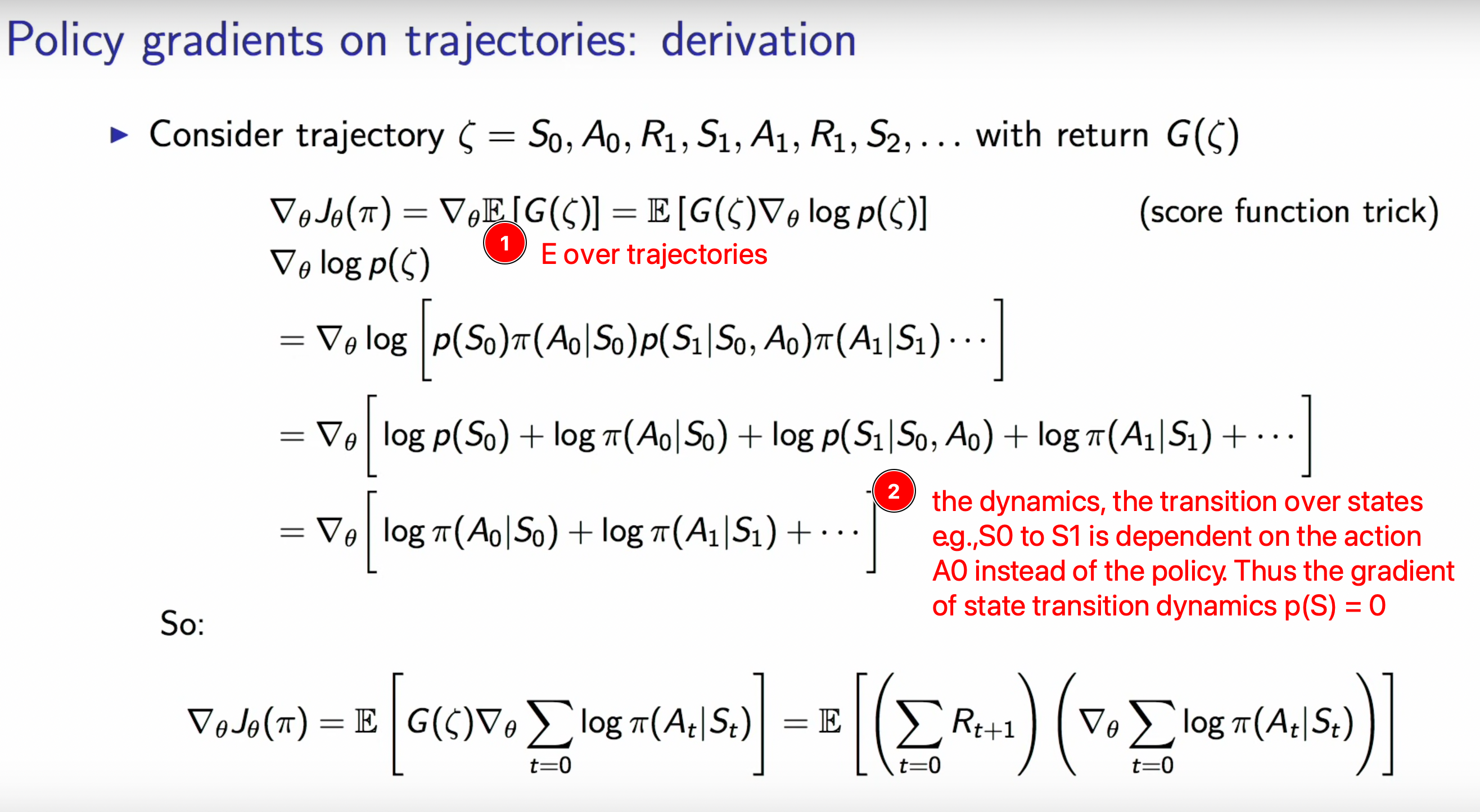
in other words, the policy only affects the decision but it doesn’t change the dynamics of the environment.
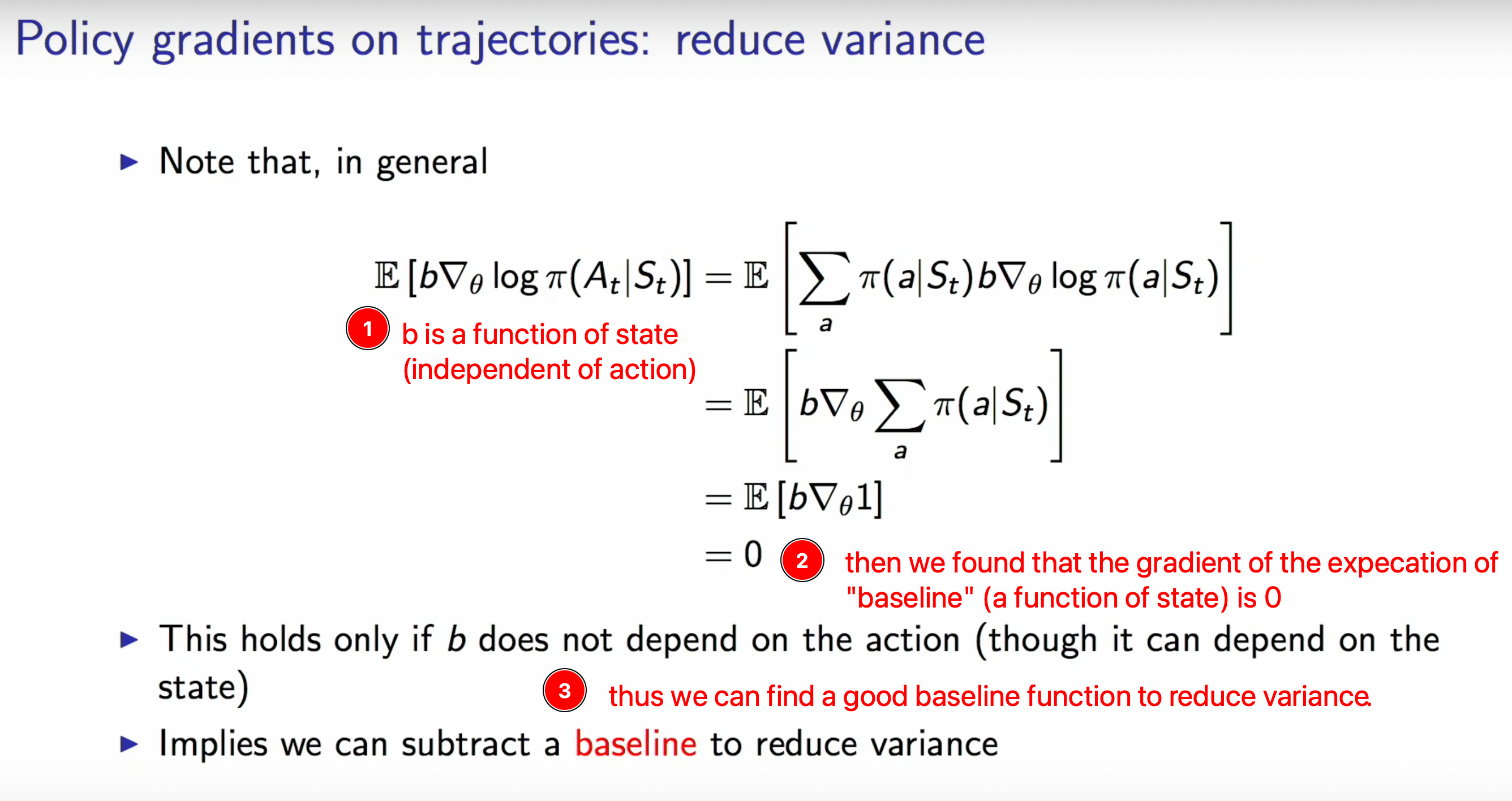
Reduce the variance to make the optimisation process more stable
E over trajectories
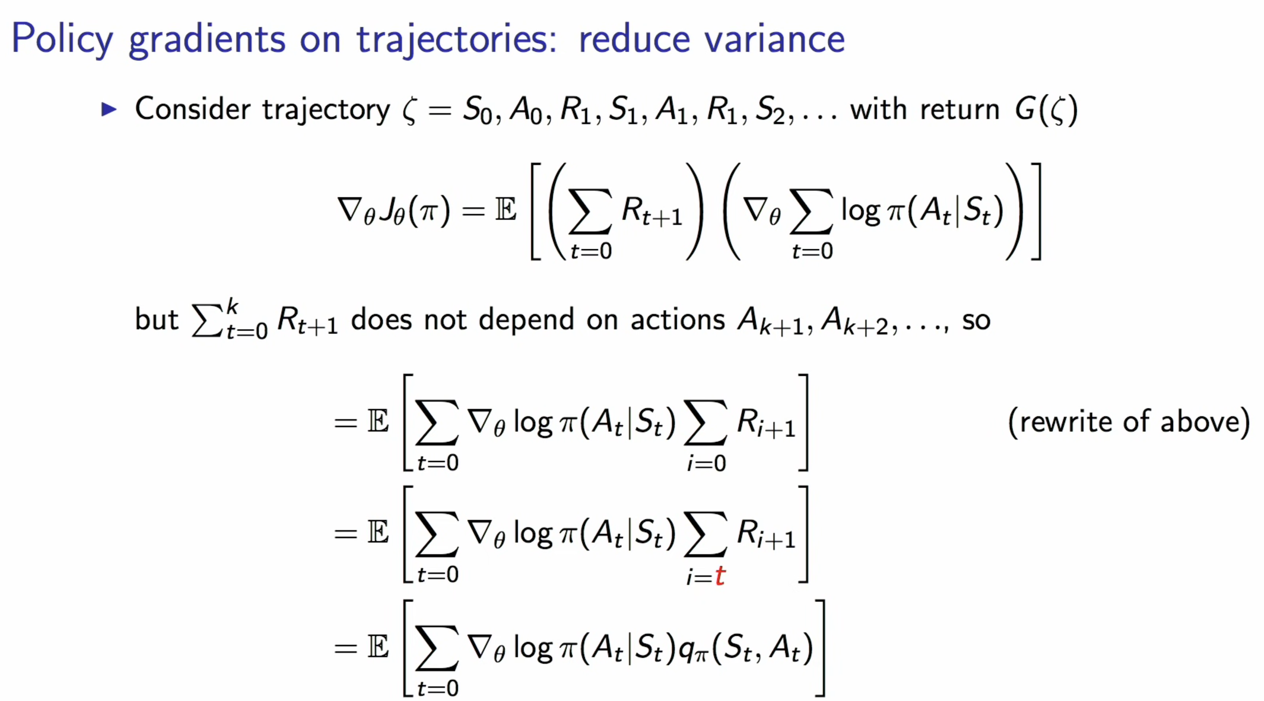
the “baseline” property allows us to remove some rewards R in the formula that is not dependent on the Action A
Continue our baseline function
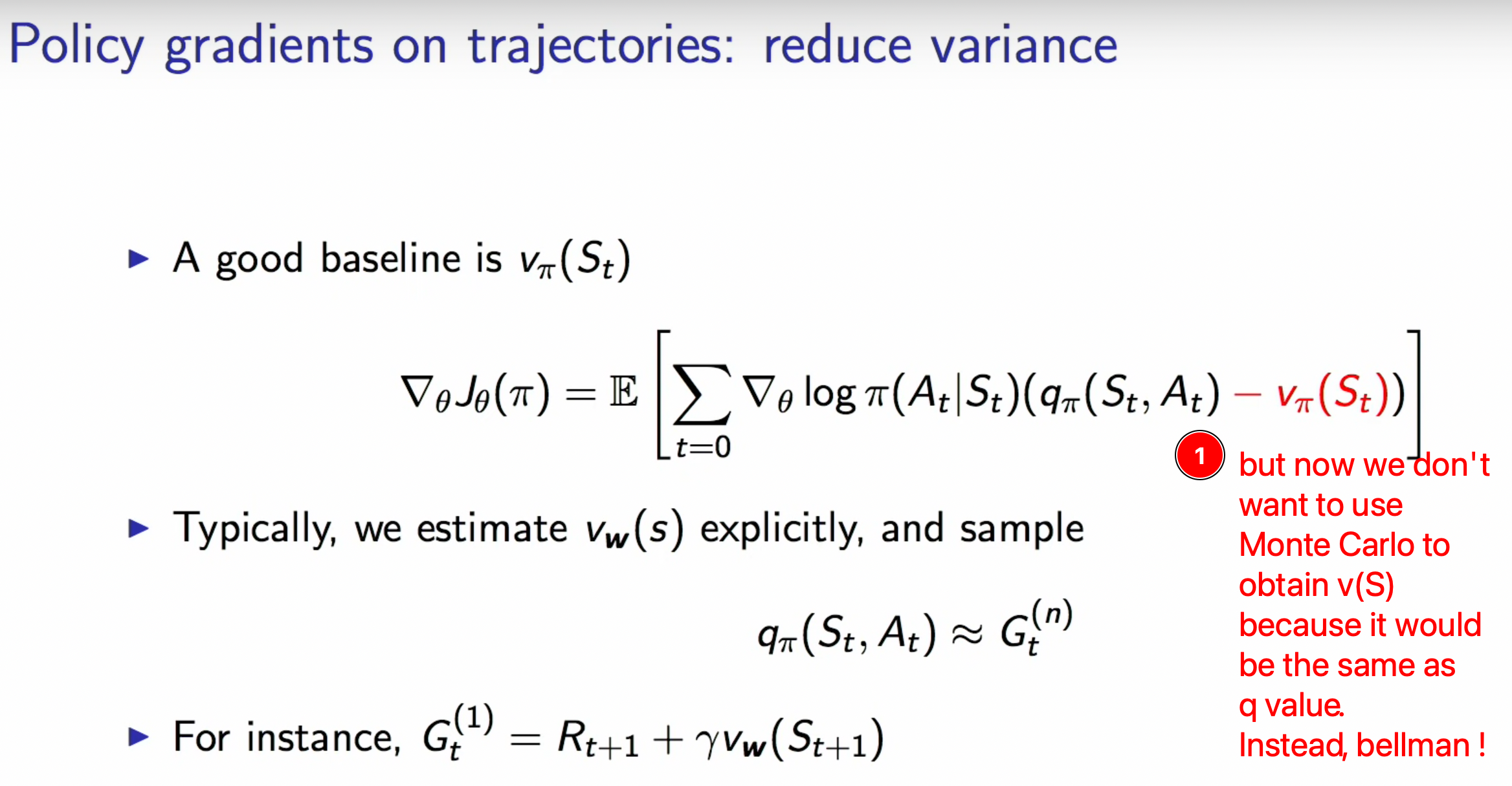
this is on policy TD learning
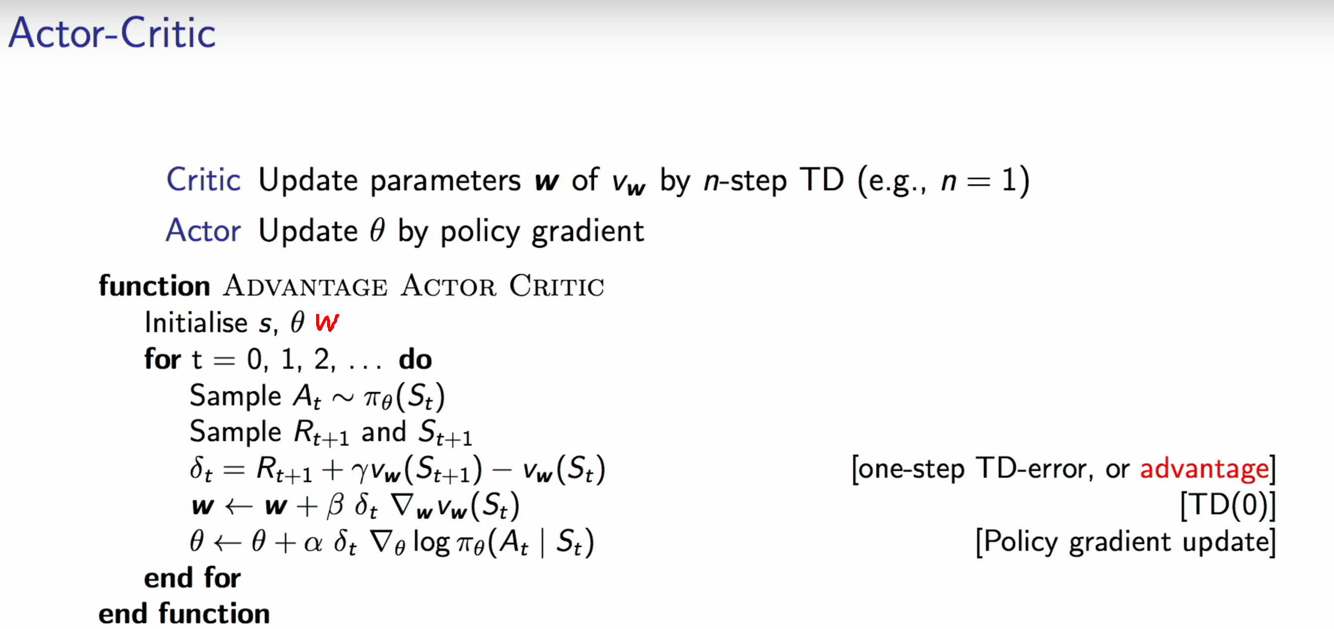
(BTW, in some cases, this is exact the same updates as Neural Q learning)
be careful of the updates, because you are changing the policy
Back to the paper
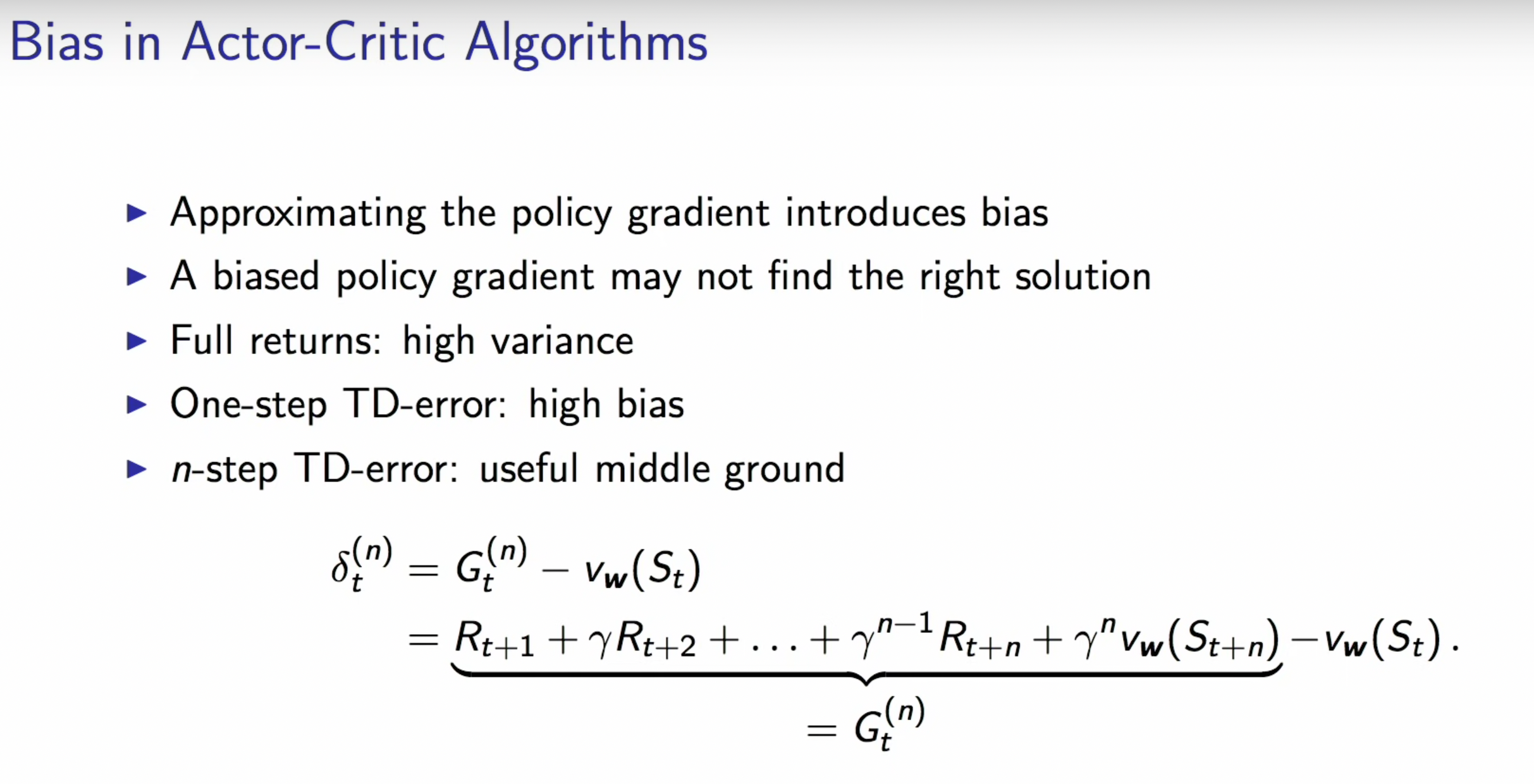
so the paper compute the gradient steps of the following form
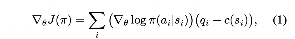
For a fixed sequence ${(s_i, a_i)}$ of states and actions obtained from a rollout of a given policy, we denote the empirical return starting in state $s_i$ as $q_i := \sum_{j=i+1} \gamma^{j-i-1}R(s_j)$
(ok, this full return would give high variance but low bias)
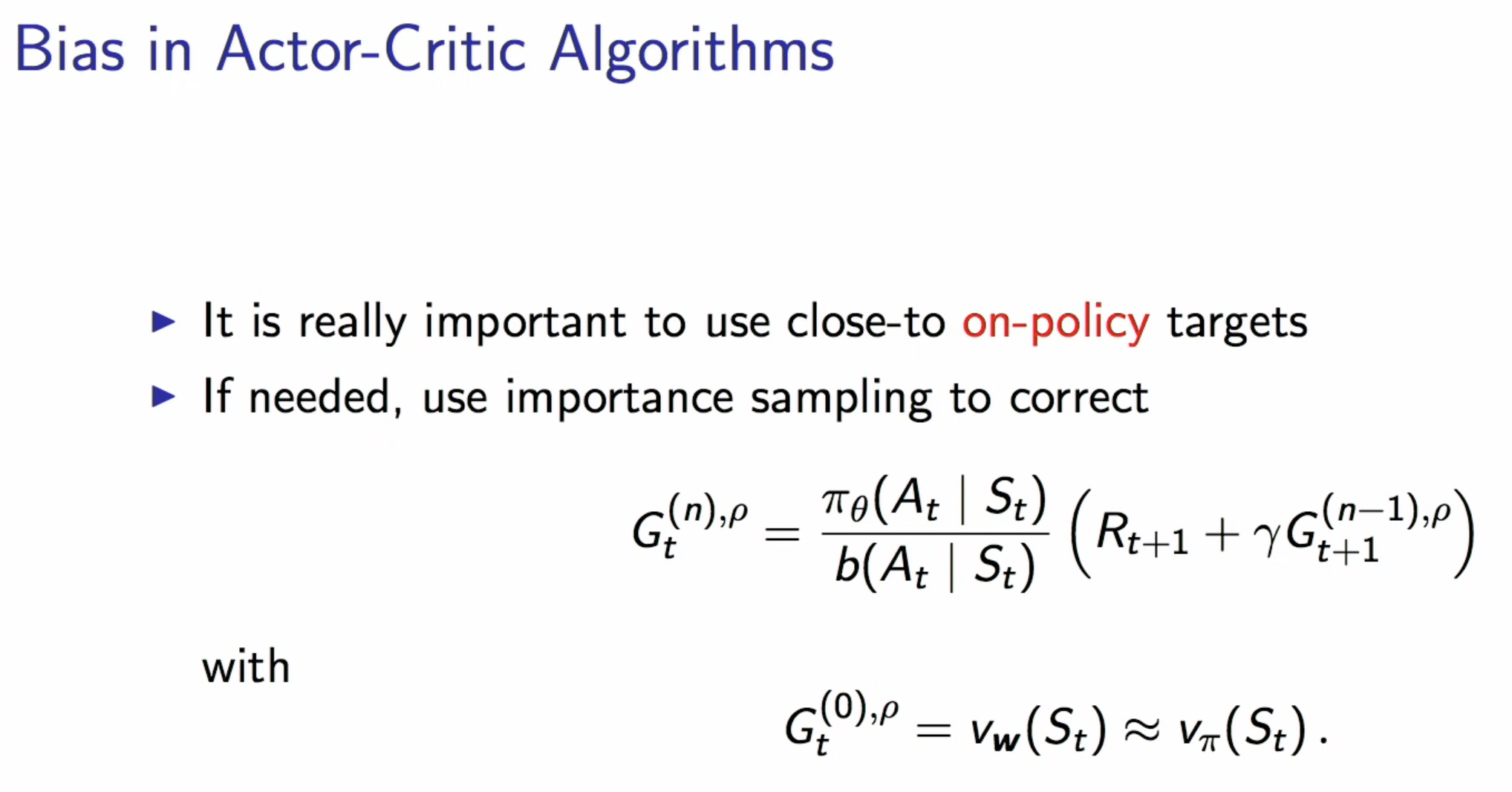
$c$ can achieve close to optimal variance when it is set exactly equal to the state value function $V_{\pi}(s_i) = \mathbf E_{\pi}q_i$ for the target policy $\pi$ starting in state $s_i$
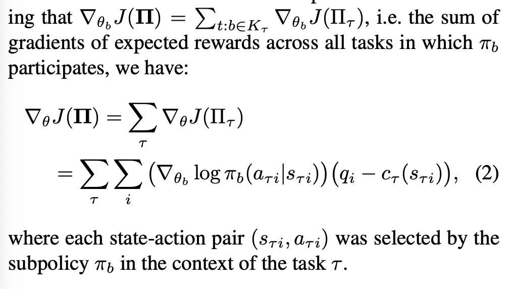
in modular policies, we only have one critic per task.
- because subpolicies $\pi_b$ might participate in a number of composed policies $\Pi_{\tau}$, each would associated with its own reward function $R_{\tau}$. Thus individual subpolicies are not uniquely identified with value functions.
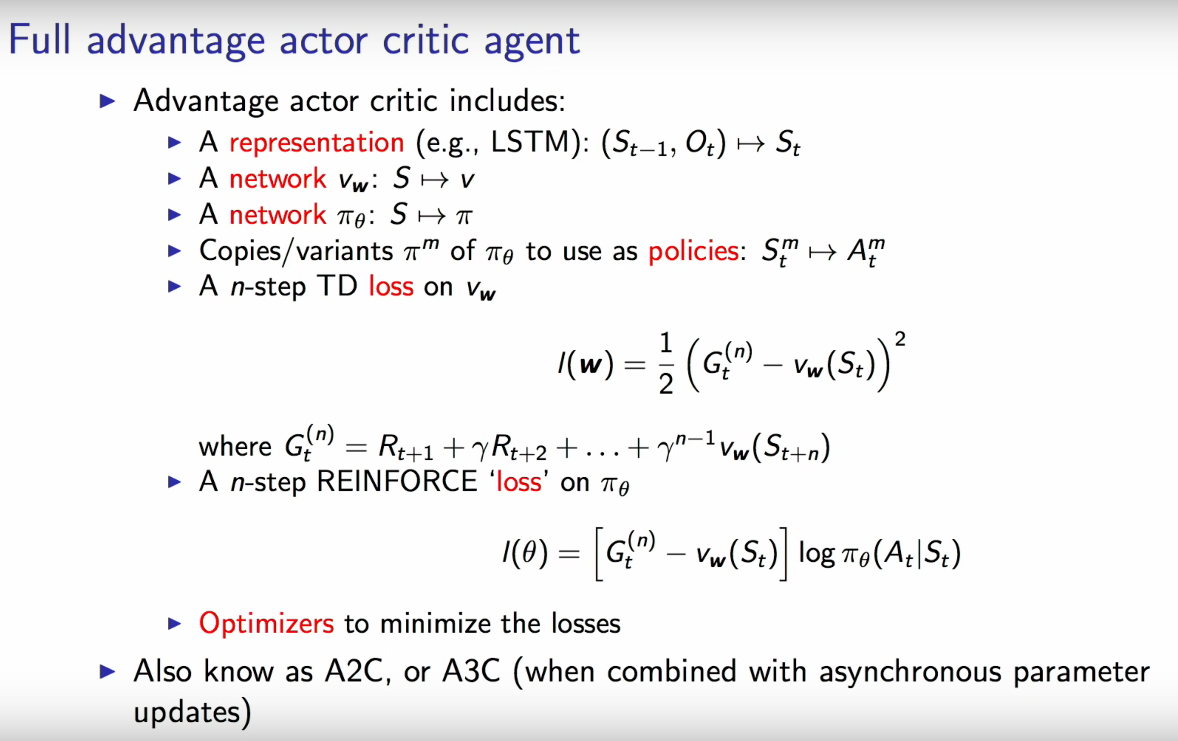
The gradient for subpolicy $\pi_{b}$
For critic, we approximate it using a network with parameters $\eta_{\tau}$
We train it by minimising a squared error criterion, with gradients given by
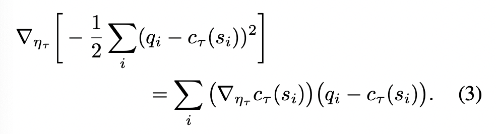
(note that this is minimisation and the previous reward on is maximisation)
note that this baseline function (i.e., critic function) is $c_{\tau}(s_i)$, thus it is dependent on both task and state identity
a complete procedure for computing a single gradient step
The complete procedure for computing a single gradient step is given as follow
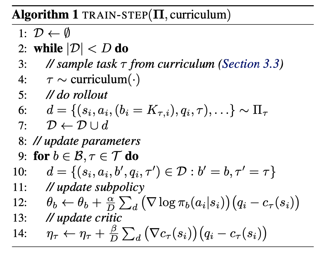
(well, we can add more stuffs to stablise the training process)
the curriculum learning
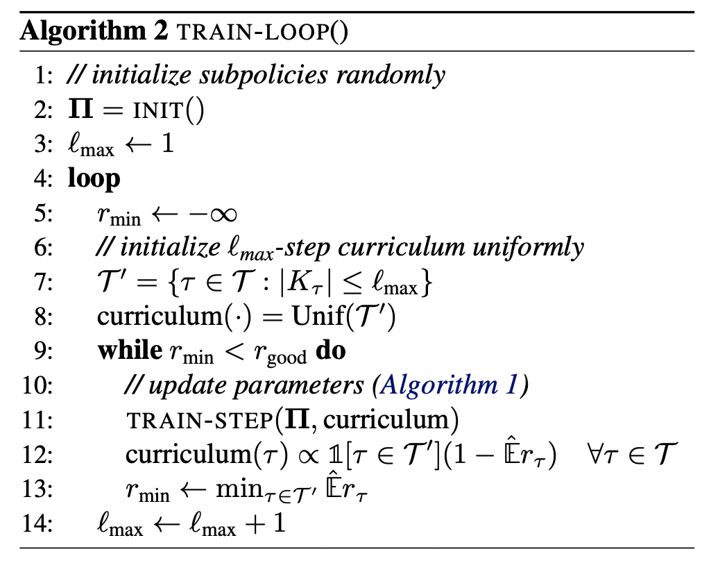
This is the part we can use “Width”