[TOC]

1. Title: SPEED: Scalable, Precise, and Efficient Concept Erasure for Diffusion Models
2. Author: Ouxiang Li, Xinting Hu et. al.
3. Publish Year: Mar 2025
4. Review Date: Wed, Apr 2, 2025
5. url: https://arxiv.org/abs/2503.07392

1

# input bibtex here

Prerequisite:

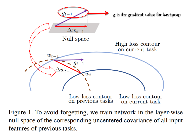
Training Networks in Null Space of Feature Covariance for Continual Learning

https://arxiv.org/abs/2103.07113

Prerequisite knowledge

projection on to a subspace of a vector

Suppose $ U = {\mathbf{u}_1, \mathbf{u}_2, \ldots, \mathbf{u}_k} $ are the orthogonal vectors spanning the subspace $ S $. Construct a matrix $ \mathbf{U} $ whose columns are these vectors: $$ \mathbf{U} = [\mathbf{u}_1 , \mathbf{u}_2 , \cdots , \mathbf{u}_k] $$ Here, $ \mathbf{U} $ is an $ n \times k $ matrix, where $ n $ is the dimension of the ambient space (e.g., $ \mathbb{R}^n $), and $ k $ is the number of basis vectors (the dimension of $ S $).

The projection of a vector $ \mathbf{v} $ onto $ S $ can then be written as: $$ \text{proj}_S \mathbf{v} = \mathbf{U} (\mathbf{U}^T \mathbf{U})^{-1} \mathbf{U}^T \mathbf{v} $$ This is the formula for the orthogonal projection onto the column space of $ \mathbf{U} $. Let’s break it down:

• $ \mathbf{U}^T $ is the transpose of $ \mathbf{U} $, a $ k \times n $ matrix.
• $ \mathbf{U}^T \mathbf{v} $ is a $ k \times 1 $ vector, computing the dot products $ \mathbf{u}_i \cdot \mathbf{v} $ for each $ i $.
• $ \mathbf{U}^T \mathbf{U} $ is a $ k \times k $ matrix, with entries $ (\mathbf{U}^T \mathbf{U})_{ij} = \mathbf{u}_i \cdot \mathbf{u}_j $. Since the $ \mathbf{u}_i $’s are orthogonal, this is a diagonal matrix with $ \mathbf{u}_i \cdot \mathbf{u}_i = |\mathbf{u}_i|^2 $ on the diagonal (and zeros off-diagonal).
• $ (\mathbf{U}^T \mathbf{U})^{-1} $ is the inverse of that diagonal matrix, so it’s also diagonal with entries $ 1 / |\mathbf{u}_i|^2 $.
• $ \mathbf{U} (\mathbf{U}^T \mathbf{U})^{-1} \mathbf{U}^T \mathbf{v} $ combines these to give the projection as a single matrix-vector product.

Why It’s Equivalent

The matrix form recovers the sum we had before. Since $ \mathbf{U}^T \mathbf{U} $ is diagonal, $ (\mathbf{U}^T \mathbf{U})^{-1} \mathbf{U}^T \mathbf{v} $ computes the coefficients $ \frac{\mathbf{v} \cdot \mathbf{u}{i}}{\mathbf{u}{i} \cdot \mathbf{u}{i}} $ for each $ \mathbf{u}{i}$, and multiplying by $ \mathbf{U} $ builds the linear combination:

$$ \mathbf{U} (\mathbf{U}^T \mathbf{U})^{-1} \mathbf{U}^T \mathbf{v} = \sum_{i=1}^k \frac{\mathbf{v} \cdot \mathbf{u}{i}}{\mathbf{u}{i} \cdot \mathbf{u}{i}} \mathbf{u}{i} $$

The orthogonality ensures $ \mathbf{U}^T \mathbf{U} $ is easy to invert (just a diagonal matrix), making this compact and computationally friendly.

Even Simpler (if Orthonormal)

If $ U $ were orthonormal (i.e., $ \mathbf{u}_i \cdot \mathbf{u}_i = 1 $ and $ \mathbf{u}_i \cdot \mathbf{u}_j = 0 $ for $ i \neq j $), then $ \mathbf{U}^T \mathbf{U} = \mathbf{I} $ (the identity matrix), and the formula simplifies further to: $$ \text{proj}_S \mathbf{v} = \mathbf{U} \mathbf{U}^T \mathbf{v} $$ But since you asked about orthogonal vectors (not necessarily orthonormal), the full form with $ (\mathbf{U}^T \mathbf{U})^{-1} $ is the most compact general expression.

Example Revisited

Take $ \mathbf{v} = [1, 2, 3] $, $ \mathbf{u}_1 = [1, 1, 0] $, $ \mathbf{u}_2 = [1, -1, 1] $: $$ \mathbf{U} = \begin{bmatrix} 1 & 1 \ 1 & -1 \ 0 & 1 \end{bmatrix} $$

• $ \mathbf{U}^T \mathbf{U} = \begin{bmatrix} 1 & 1 & 0 \ 1 & -1 & 1 \end{bmatrix} \begin{bmatrix} 1 & 1 \ 1 & -1 \ 0 & 1 \end{bmatrix} = \begin{bmatrix} 2 & 0 \ 0 & 3 \end{bmatrix} $ (since $ \mathbf{u}_1 \cdot \mathbf{u}_1 = 2 $, $ \mathbf{u}_2 \cdot \mathbf{u}_2 = 3 $, and $ \mathbf{u}_1 \cdot \mathbf{u}_2 = 0 $).
• $ (\mathbf{U}^T \mathbf{U})^{-1} = \begin{bmatrix} \frac{1}{2} & 0 \ 0 & \frac{1}{3} \end{bmatrix} $
• $ \mathbf{U}^T \mathbf{v} = \begin{bmatrix} 3 \ 2 \end{bmatrix} $ (from dot products).
• $ (\mathbf{U}^T \mathbf{U})^{-1} \mathbf{U}^T \mathbf{v} = \begin{bmatrix} \frac{1}{2} & 0 \ 0 & \frac{1}{3} \end{bmatrix} \begin{bmatrix} 3 \ 2 \end{bmatrix} = \begin{bmatrix} \frac{3}{2} \ \frac{2}{3} \end{bmatrix} $
• $ \mathbf{U} (\mathbf{U}^T \mathbf{U})^{-1} \mathbf{U}^T \mathbf{v} = \begin{bmatrix} 1 & 1 \ 1 & -1 \ 0 & 1 \end{bmatrix} \begin{bmatrix} \frac{3}{2} \ \frac{2}{3} \end{bmatrix} = [\frac{13}{6}, \frac{7}{6}, \frac{2}{3}] $, matching the sum method.

Final Compact Form

So, the projection is: $$ \text{proj}_S \mathbf{v} = \mathbf{U} (\mathbf{U}^T \mathbf{U})^{-1} \mathbf{U}^T \mathbf{v} $$ This avoids the summation symbol, encapsulates everything in matrix operations, and scales nicely for any number of orthogonal vectors. It’s a sleek, elegant way to express the same idea—perfect for linear algebra enthusiasts!

Null space and Covariance Matrix

Let’s dive into why $ C v_i = 0 $ when $ v_i $ is a null vector, specifically in the context of a covariance matrix $ C $ and its relationship to Singular Value Decomposition (SVD). This ties back to our earlier discussions, so I’ll build on that foundation and keep it clear and logical.

Setting the Stage

• Covariance Matrix $ C $: Assume $ C $ is the uncentered covariance matrix of a data matrix $ X $ (with $ m $ observations and $ n $ features), defined as: $$ C = \frac{1}{m} X^T X $$ $ C $ is an $ n \times n $ symmetric, positive semi-definite matrix.
• Null Vector: A vector $ v_i $ is in the null space of $ C $ if $ C v_i = 0 $. The null space consists of all vectors that $ C $ maps to the zero vector.
• SVD of $ X $: $ X = U \Sigma V^T $, where:
  • $ U $ is $ m \times m $ (left singular vectors),
  • $ \Sigma $ is $ m \times n $ (diagonal matrix of singular values $ \sigma_1, \sigma_2, \dots $),
  • $ V $ is $ n \times n $ (right singular vectors, with columns $ v_1, v_2, \dots, v_n $).

Connecting $ C $ to SVD

First, express $ C $ using the SVD of $ X $: $$ X^T X = (U \Sigma V^T)^T (U \Sigma V^T) = V \Sigma^T U^T U \Sigma V^T $$ Since $ U $ is orthogonal ($ U^T U = I $): $$ X^T X = V \Sigma^T \Sigma V^T $$ Thus: $$ C = \frac{1}{m} X^T X = \frac{1}{m} V \Sigma^T \Sigma V^T $$

• $ \Sigma^T \Sigma $ is an $ n \times n $ diagonal matrix with entries $ \sigma_i^2 $ (squared singular values) on the diagonal and zeros elsewhere.
• $ V $ is orthogonal ($ V^T V = I $), and its columns $ v_i $ are the eigenvectors of $ X^T X $ (and thus of $ C $).
• The eigenvalues of $ C $ are $ \lambda_i = \frac{\sigma_i^2}{m} $.

Why $ C v_i = 0 $ for a Null Vector

A vector $ v_i $ is a null vector of $ C $ if $ C v_i = 0 $. Let’s see how this happens:

1. Apply $ C $ to $ v_i $: $$ C v_i = \left( \frac{1}{m} V \Sigma^T \Sigma V^T \right) v_i $$ Since $ v_i $ is a column of $ V $ (say the $ i $-th column), and $ V $ is orthogonal: $$ V^T v_i = e_i $$ where $ e_i $ is the $ i $-th standard basis vector (all zeros except a 1 in the $ i $-th position).

2. Multiply by $ \Sigma^T \Sigma $: $$ \Sigma^T \Sigma V^T v_i = \Sigma^T \Sigma e_i $$

   • $ \Sigma^T \Sigma $ is diagonal, with entries $ \sigma_1^2, \sigma_2^2, \dots, \sigma_n^2 $.
   • Multiplying $ \Sigma^T \Sigma $ by $ e_i $ picks out the $ i $-th diagonal element: $$ \Sigma^T \Sigma e_i = \sigma_i^2 e_i $$

3. Multiply by $ V $: $$ C v_i = \frac{1}{m} V (\Sigma^T \Sigma e_i) = \frac{1}{m} V (\sigma_i^2 e_i) $$

   • $ V e_i = v_i $ (since $ e_i $ extracts the $ i $-th column of $ V $).
   • So: $$ C v_i = \frac{1}{m} \sigma_i^2 v_i $$

4. Condition for Null Vector:

   • For $ C v_i = 0 $ to hold: $$ \frac{1}{m} \sigma_i^2 v_i = 0 $$
   • Since $ \frac{1}{m} \neq 0 $ and $ v_i \neq 0 $ (it’s a non-zero vector as a column of $ V $), this is true if and only if: $$ \sigma_i^2 = 0 \quad \text{or equivalently,} \quad \sigma_i = 0 $$
   • Thus, $ v_i $ is a null vector of $ C $ when its corresponding singular value $ \sigma_i = 0 $.

Eigenvalue Perspective

Since $ C = \frac{1}{m} V \Sigma^T \Sigma V^T $ is the eigen decomposition of $ C $:

• $ v_i $ is an eigenvector of $ C $.
• The corresponding eigenvalue is $ \lambda_i = \frac{\sigma_i^2}{m} $.
• If $ \sigma_i = 0 $, then $ \lambda_i = 0 $, and: $$ C v_i = \lambda_i v_i = 0 \cdot v_i = 0 $$ This confirms that $ v_i $ being in the null space corresponds to a zero eigenvalue, which happens when $ \sigma_i = 0 $.

Intuition

• Geometric View: The singular value $ \sigma_i $ measures the “stretch” of $ X $ along the direction $ v_i $ in the feature space. If $ \sigma_i = 0 $, $ X $ has no variation in that direction—all data points project to zero along $ v_i $. For the uncentered covariance matrix, this means the raw data lies entirely in a subspace orthogonal to $ v_i $.
• Data Example: If $ X = \begin{bmatrix} 1 & 1 \ 1 & 1 \end{bmatrix} $, the second singular vector $ v_2 = \begin{bmatrix} -\frac{1}{\sqrt{2}} \ \frac{1}{\sqrt{2}} \end{bmatrix} $ has $ \sigma_2 = 0 $, and $ C v_2 = 0 $, because the data has no variation in that direction (all rows are identical).

Why It Happens

$ C v_i = 0 $ when $ v_i $ is a null vector because:

• $ v_i $ is a right singular vector of $ X $ with a zero singular value ($ \sigma_i = 0 $).
• This zero singular value indicates no variance in the direction of $ v_i $ in the data.
• The covariance matrix $ C $, being derived from $ X^T X $, reflects this by mapping $ v_i $ to zero, placing it in the null space.

In short, $ C v_i = 0 $ because $ v_i $ corresponds to a direction where the data (via $ X $) has no spread, and SVD neatly identifies these directions through zero singular values.

Covariance Matrix and its semantic

In the context of your question and our previous discussion about covariance matrices and SVD, the term “variable” typically refers to a feature, not an observation. Let me clarify the distinction and how it applies here:

Definitions

• Feature (Variable): A feature is a measurable property or characteristic of the data, often represented as a column in a data matrix. For example, in a dataset about people, features might be height, weight, or age. In statistics and machine learning, “variable” is often synonymous with “feature” when discussing datasets.
• Observation: An observation is an individual data point or instance, typically represented as a row in a data matrix. It’s a single measurement of all features for one entity (e.g., one person’s height, weight, and age).

In the Context of a Data Matrix

Suppose you have a data matrix $ X $ with $ m $ rows and $ n $ columns:

• $ m $: Number of observations (e.g., number of people).
• $ n $: Number of features/variables (e.g., height, weight, etc.).
• $ X $ is $ m \times n $, where each column corresponds to a feature (variable) and each row corresponds to an observation.

For example: $$ X = \begin{bmatrix} 160 & 60 & 7 \ 165 & 65 & 8 \ 170 & 70 & 9 \end{bmatrix} $$

• Rows (3 observations): Each row is a person.
• Columns (3 features/variables): Height, weight, shoe size.

Covariance Matrix and Variables

The covariance matrix $ C $ is computed over the features (variables): $$ C = \frac{1}{m-1} X^T X \quad \text{(centered)} \quad \text{or} \quad C = \frac{1}{m} X^T X \quad \text{(uncentered)} $$

• $ C $ is $ n \times n $, where $ n $ is the number of features.
• The diagonal of $ C $ gives the variance of each feature (e.g., variance of height, variance of weight).
• The off-diagonal elements give the covariance between pairs of features (e.g., covariance between height and weight).

So, in this context, “variable” refers to a feature (a column of $ X $), not an observation.

SVD Context

In SVD ($ X = U \Sigma V^T $):

• $ V $ (right singular vectors) corresponds to the feature space (variables).
• $ U $ (left singular vectors) corresponds to the observation space.
• The covariance matrix $ C $ relates to $ V $ because $ X^T X = V \Sigma^T \Sigma V^T $, and $ V $’s columns are the eigenvectors of $ C $, describing directions in the feature (variable) space.

Answering Your Question

“Is variable feature or observation?”

• Variable = Feature. In the discussions we’ve had (covariance matrix, SVD, null space), “variable” refers to a feature (a column in $ X $), not an observation (a row in $ X $).

Summary of paper

Motivation

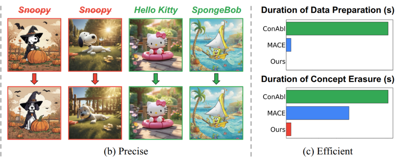
This paper introduces SPEED, a novel editing-based method for concept erasure in text-to-image (T2I) diffusion models. SPEED addresses the key challenge of balancing erasure efficacy with preservation of non-target semantics (prior preservation). It incorporates null-space constraints for model editing, and introduces three key innovations: Influence-based Prior Filtering (IPF), Directed Prior Augmentation (DPA), and Invariant Equality Constraints (IEC). The method achieves scalable and efficient erasure, outperforming existing techniques across multiple tasks (e.g., multi-concept, implicit concept erasure), and demonstrates 350× speedup over state-of-the-art.

Contribution

Technical Novelty:

• The use of null-space projection to minimize non-target drift is theoretically sound and well-justified.
• IPF identifies key non-targets affected by erasure, improving the retain set selection adaptively.
• DPA improves on random augmentation by introducing semantically meaningful variations.
• IEC cleverly leverages architectural invariants to preserve critical components of the generation pipeline.

Some key terms

What is training-free editing-based paradigm for concept erasing

• it jointly optimizes erasure and preservation objectives for target and non-target concept (contrastive samples!) in a closed-form solution, obtaining direct modification over model parameters
  • e.g., projection weights in cross-attention layer
• some objective is bad
  • e.g., weighted least squares optimization will always imposing a non-zero lower bound on preservation error.

What is null space

• the subspace that does not alter the feature representation of non-target concepts
• By projecting the model parameter updates for erasing concepts onto the null space of non-target concepts, SPEED can minimize the preservation error close to zero without compromising erasure efficacy.

[!IMPORTANT]

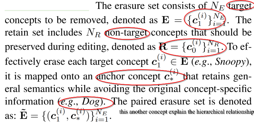
But what if the relationship between non-target and target are in hierarchical relationship? (human and mammal )

In the context of null space construction refers to the situation where the matrix used to define the null space (often from a set of vectors you want to preserve) becomes full rank, thereby shrinking or eliminating the null space entirely.

Let’s break it down in simple terms:

❓ What is the null space?

In linear algebra, the null space of a matrix $ A $ is the set of all vectors $ x $ such that: $$ Ax = 0 $$

In this paper (SPEED), the matrix $ C_0 $ is built from non-target concept embeddings (concepts you want to preserve). The null space of $ C_0 $ is used to find directions where modifications (i.e., concept erasure updates) don’t interfere with these preserved concepts.

💥 What is rank saturation?

• The rank of $ C_0 $ is the number of linearly independent vectors in the retain set.
• The null space gets smaller as the rank of $ C_0 $ increases.
• If the rank of $ C_0 $ equals the dimension of the space (i.e., full rank), then the null space becomes trivial — it only contains the zero vector.

This is called rank saturation — you’ve added so many concepts to preserve that there’s no more “safe space” left for edits (the null space is zero-dimensional).

⚠️ Why is this a problem in SPEED?

• SPEED projects edits onto the null space of $ C_0 $ to preserve the non-target concepts.
• But if the retain set becomes too large or too diverse, $ C_0 $ becomes full-rank, and the null space collapses.
• This means you can no longer update the model without affecting at least one non-target concept — so preservation breaks down.

🛠️ How does SPEED fix this?

SPEED introduces:

• IPF to filter only the most affected non-targets.
• DPA to augment the retain set intelligently using semantically similar embeddings — so they don’t add too much rank.
• These steps ensure that the null space remains non-trivial and useful for concept erasure without corrupting preserved knowledge.

Method

target, anchor and non-target

[!IMPORTANT]

This anchor vectors explain the hierarchical relationship concern

Goal of concept erase

You have a target concept embedding $ c_1 $ (e.g., “Snoopy”) that you want to erase, and replace it with a more generic or neutral anchor concept $ c^* $ (e.g., “Dog”).

You want the model’s updated behavior to treat $ c_1 $ like $ c^* $. So we want the updated weights to satisfy: $$ (W + \Delta) c_1 \approx W c^* $$

This leads to the erasure objective:
Minimize the difference between what the model used to do with the anchor and what it will do with the erased concept after the update: $$ e_1 = | (W + \Delta) c_1 - W c^* |^2 $$

Why does $ \Delta \cdot c_0 \ne 0 $ mean that the weight update impacts $ c_0 $?

This boils down to how linear transformations work in neural networks — especially in the cross-attention layers of diffusion models where these concepts live.

Let’s walk through it clearly:

🔁 Recap: What is $ \Delta \cdot c_0 $ in context?

• $ \Delta $: the change you’re making to a model weight matrix (like a projection matrix in attention).
• $ c_0 $: a non-target concept embedding (e.g., “Mickey”).

So, $ \Delta \cdot c_0 $ is the change in the model’s output when inputting the concept $ c_0 $ — caused solely by your weight update.

🧠 Why does it mean “impact”?

Because in linear models, output = weight × input.

So, if the original model had: $$ W \cdot c_0 = \text{some output} $$ and you apply an update $ \Delta $, the new output becomes: $$ (W + \Delta) \cdot c_0 = W \cdot c_0 + \Delta \cdot c_0 $$

So:

• The change in output is: $$ \text{new output} - \text{old output} = \Delta \cdot c_0 $$

Therefore:

• If $ \Delta \cdot c_0 = 0 $, then the model’s output for $ c_0 $ hasn’t changed
• If $ \Delta \cdot c_0 \ne 0 $, then the model’s output for $ c_0 $ has changed

That’s why we say $ \Delta \cdot c_0 $ measures how much impact your update has on $ c_0 $

🧮 Analogy

Imagine you have a function $ f(x) = Wx $, and you perturb $ W $ to $ W + \Delta $. Now:

• $ f_{\text{old}}(x) = Wx $
• $ f_{\text{new}}(x) = (W + \Delta)x = Wx + \Delta x $

That extra $ \Delta x $ is the effect of your update on the output. If it’s not zero, you’ve changed the function’s behavior on $ x $.

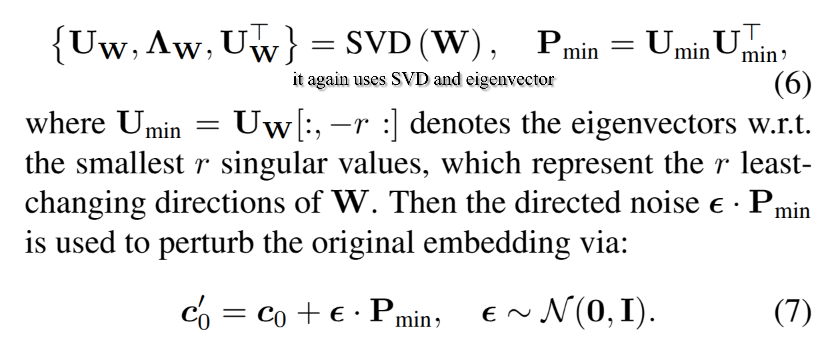
DPA

After IPF, do data augmentation to have diversity of the retrain set, but not increasing the null space as they are semantic similar

Introduce directed noise by projecting the random noise $\epsilon$ on the direct in which the model parameter $\textbf{W}$ exhibit minimal variation

IEC

“Hard equality constraint means that the update of weights are in the null space of $ C_2 $, and thus will not impact $ C_2 $”

$C_2$ is the feature stack matrix where the features are those we do not want to change, e.g., [SOT] start of text token

What are Lagrange Multipliers?

Lagrange multipliers are a method from optimization theory used to solve constrained optimization problems. Specifically:

Minimize some function $ f(x) $,
subject to equality constraints: $ g(x) = 0 $

We introduce a Lagrange multiplier $ \lambda $, and define a new function (the Lagrangian): $$ \mathcal{L}(x, \lambda) = f(x) + \lambda^\top g(x) $$

Then we find the stationary point by solving: $$ \nabla_x \mathcal{L} = 0 \quad \text{and} \quad g(x) = 0 $$ $g(x) = 0$ is a hard constraint — not just a preference. We must enforce it.

But in regular unconstrained optimization (like gradient descent), we can’t do this easily. So we use Lagrange multipliers to turn it into one function that combines both the objective and the constraint.

🔍 What is $ \Lambda $ in this context?

In SPEED’s constrained optimization:

• $ \Delta $: weight update (what we’re solving for)
• Constraint: $ (\Delta P) C_2 = 0 $ — don’t affect invariant embeddings
• $ \Lambda $: the matrix of Lagrange multipliers, one column per constraint (one per column in $ C_2 $)

So:

• $ \Lambda $ tells you how “costly” it is (in terms of increased loss) to enforce each constraint.

✨ Interpretations of $ \Lambda $

Sensitivity of the objective to the constraint

Each component of $ \Lambda $ corresponds to how much the final loss would increase if you relaxed the corresponding constraint just a bit.

So:

• A large magnitude in $ \Lambda $ for a column $ c_2^{(i)} \in C_2 $ means:

  The constraint on that invariant is really tight — the optimizer had to work hard to keep it satisfied, and relaxing it would lower the loss significantly.

• A small or zero $ \Lambda $ means:

  That invariant was easy to preserve — it didn’t interfere much with erasure.

Shape